Measurement and uncertainty

Bayesian Methods for Ecological and Environmental Modelling

Peter Levy
UKCEH Edinburgh

Recap

Recap

• Bayesian basics
  • inference using conditional probability
• MCMC
  • how to implement Bayesian inference
• Linear Modelling
  • Bayesian estimation of simple model parameters
  • \(y = \alpha + \beta x + \epsilon\)

Recap

• Model selection & comparison
  • how to choose between competing models

Questions?

Measurement and uncertainty

Terminology for measurements

• “The Facts”
• Evidence
• Observations
• Measurements
• Data

Terminology for measurements

• “The Facts”
• Evidence
• Observations
• Measurements
• Data

All the same thing, increasing uncertainty.

Measurements and uncertainty

Measurements are a proxy for true process of interest. Connection between the two can be:

• sample from population (sampling error)
• imperfect measurements (measurement error)

Measurements and uncertainty

Measurements are a proxy for true process of interest. Connection between the two can be:

• proxy variables
  • true variable is hard to measure but can be approximated

Measuring stream flow

The stream flow rate \(Q\) is the product of the stream cross-sectional area and its velocity. A pressure transducer continuously records stream height \(h\) via the pressure, \(P_{\mathrm{stream}}\).

Measuring streamflow

• We would typically say we have “measurements of streamflow”
• But we actually have measurements of stream height
• or rather water pressure …
• or rather pressure transducer output voltage …
• or rather data logger measurements of voltage.

Streamflow example

We have a series of four linear models:

\[\begin{align*} Q_{flow} =& \beta_1 + \beta_2 h_{stream} + \epsilon_1 \\ h_{stream} =& \beta_3 + \beta_4 P_{sensor} + \epsilon_2 \\ P_{sensor} =& \beta_5 + \beta_6 V_{sensor} + \epsilon_3 \\ V_{sensor} =& \beta_7 + \beta_8 V_{logger} + \epsilon_4 \end{align*}\]

We effectively assume these models are perfect and the error terms \(\epsilon\) 1-4 are zero.

This is a relatively simple case, and some of these errors may well be negligible. Many cases are not so simple.

Streamflow example

We can substitute one model in another:

\[\begin{align*} \label{eq:strr} Q_{flow} =& \beta_1 + \beta_2 (\beta_3 + \beta_4 P_{sensor} + \epsilon_2) + \epsilon_1 \\ P_{sensor} =& \beta_5 + \beta_6 V_{sensor} + \epsilon_3 \\ V_{sensor} =& \beta_7 + \beta_8 V_{logger} + \epsilon_4 \end{align*}\]

to give a single model:

\[\begin{align*} \label{eq:stream3} Q_{flow} = \beta_1 +& \beta_2 (\beta_3 + \beta_4 (\beta_5 + \beta_6 (\beta_7 + \beta_8 V_{logger} \\ +& \epsilon_4) + \epsilon_3) + \epsilon_2) + \epsilon_1 \end{align*}\]

Measurements and uncertainty

Measurements are a proxy for true process of interest. Connection between the two can be:

• proxy variables
  • true variable is hard to measure but can be approximated

Measurements and uncertainty

Measurements are a proxy for true process of interest. Connection between the two can be:

• proxy variables
  • true variable is hard to measure but can be approximated

Measurements and uncertainty

Measurements are a proxy for true process of interest. Connection between the two can be:

• proxy variables
  • true variable is hard to measure but can be approximated

Uncertainty in upscaling

Often, true process of interest is a larger-scale property (e.g. annual sum, regional mean)

• integration
• interpolation / extrapolation,
• accounting for small-scale heterogeneity
• adds additional modelling steps

Ignoring measurement error has consequences

But uncertainty often not propagated. Leads to results with:

1. under-reported random uncertainty
   • low statistical power
   • low true positive rate
2. under-reported systematic uncertainty
   • biases, artefacts
   • high false positive rate

Ignoring measurement error has consequences

But uncertainty often not propagated. Leads to:

• high “false discovery rate”
  • P(claiming to find effect when none present)
• biased results in literature

The Reproducibility Crisis

Understanding false discovery rates

“Why most published research findings are false”

High “false discovery rates”, often much higher than 5 %

1. Low prior probabilities - unlikely / rare effects
2. Low statistical power - low signal:noise
3. Bias - systematic uncertainties in observation process

Crux of Ioannidis’ paper was high FDR

3 reasons, last two common in ecology

1. Low prior probabilities

First of these is the same as the medical screening paradox - familiar from covid

Disesaes are rare in the population - say 1%

Take 1000 people, only 10 will have it

One example of same phenomenon in ecology - LUC

Also spp ID from AI

Example: Land-use change

Suppose satellite covers 100,000 km2 forest

and you are looking for deforestation - rare in Europe - all same logic applies

Empirical evidence from UK study

2. Low statistical power

What if effect is common but power is low?

Power is true positive rate.

Here, we have low denominator, so FDR relatively high

2. Effect of low power

All predictable with simple calculation

2. Low power in ecology

• large background variability cf. effect size
• difficulty of measurement
• small sample size
• measurement error
• measurements are a proxy for true process of interest
  • error not propagated

Low power common in ecology

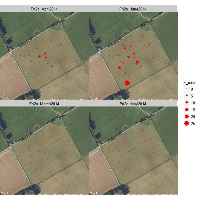
Example: gas emissions from soil

One example - point is mmnt is difficult

Spatial variation in gas emissions

We need cumulative emissions

3. Bias in observation process

Lastly, bias affects numerator

Anything which could differ systematically between treatments

The point of experiments is to avoid this

But sometimes not possible in ecology

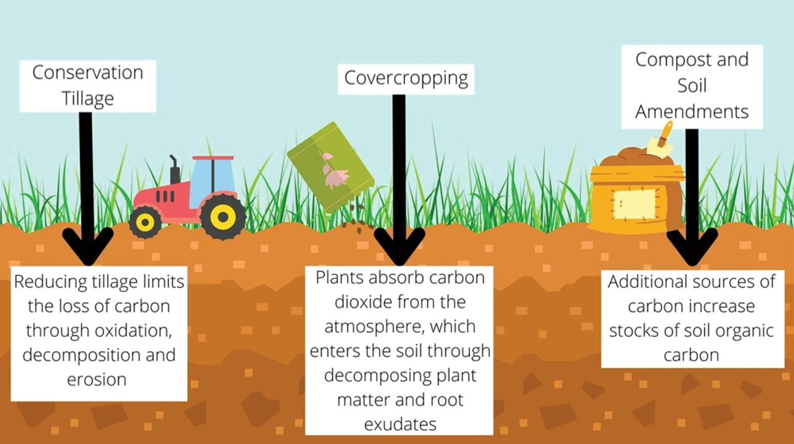
Example: soil carbon change

Example: alot of interest in carbon credits

But takes 10 years to detect change

and hard to avoid bias

Even et al, 2024, Biogeosciences.

3. Effect of bias

Example: Soil carbon change

Motivation: increasing carbon sequestration in the soil is a potential means to offset greenhouse gas emissions

• farmers can be paid for land management which achieves this
  • cover crops, organic manure, reduced ploughing etc.
• detectable as in increase in soil carbon stock
• payments should reflect actual outcomes

Measuring soil carbon: field

Take soil cores

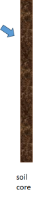
Measuring soil carbon: lab

Soil carbon: integrate over depth

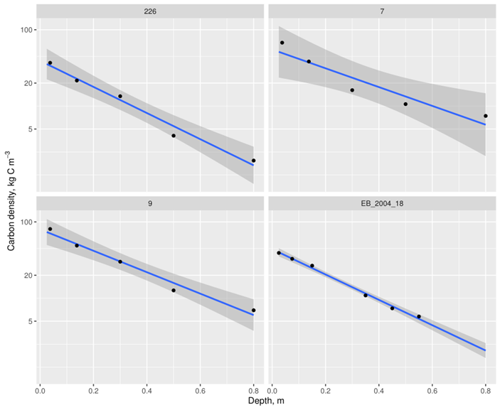
\(\mathrm{log} C = \alpha + \beta \times \mathrm{depth}\)

Soil carbon: integrate over space

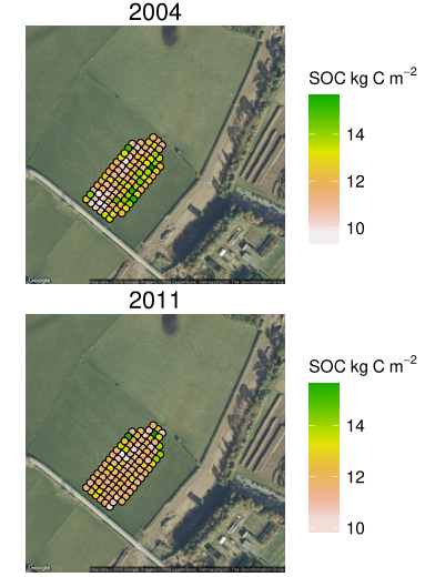
Extrapolate samples to whole field with spatial model

\(\mu_{\mathrm{field}} = f(\theta, C_{\mathrm{samples}})\)

Soil carbon: uncertainties

• We would typically say we have “measurements of soil carbon”.
• But we actually have measurements of weight loss
• from a sample of a sample …
• from which we predict carbon fraction with a model …
• and predict carbon stock to depth with a model …
• and extrapolate this in space with a model …
• and we (usually) ignore most of the uncertainties!

Soil carbon: uncertainties

It gets worse.

• Systematic uncertainties (bias) from different:
• surveyors
• sampling protocols
• areas & depths sampled
• labs & instruments
• lab protocols
• very hard to be consistent over ~20 years.

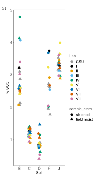
Soil carbon: same soil, different labs

Soil carbon: real data

Soil carbon: real data

Practical

Estimating false discovery rates

Propagating uncertainty

“Why most published research findings are false” - the other reasons

“Why most published research findings are false”

• “The garden of forking paths”
  • many possible choices in data collection & analysis
  • choices favour finding interesting patterns
• Motivated cognition
  • “the influence of motives on memory, information processing & reasoning.”

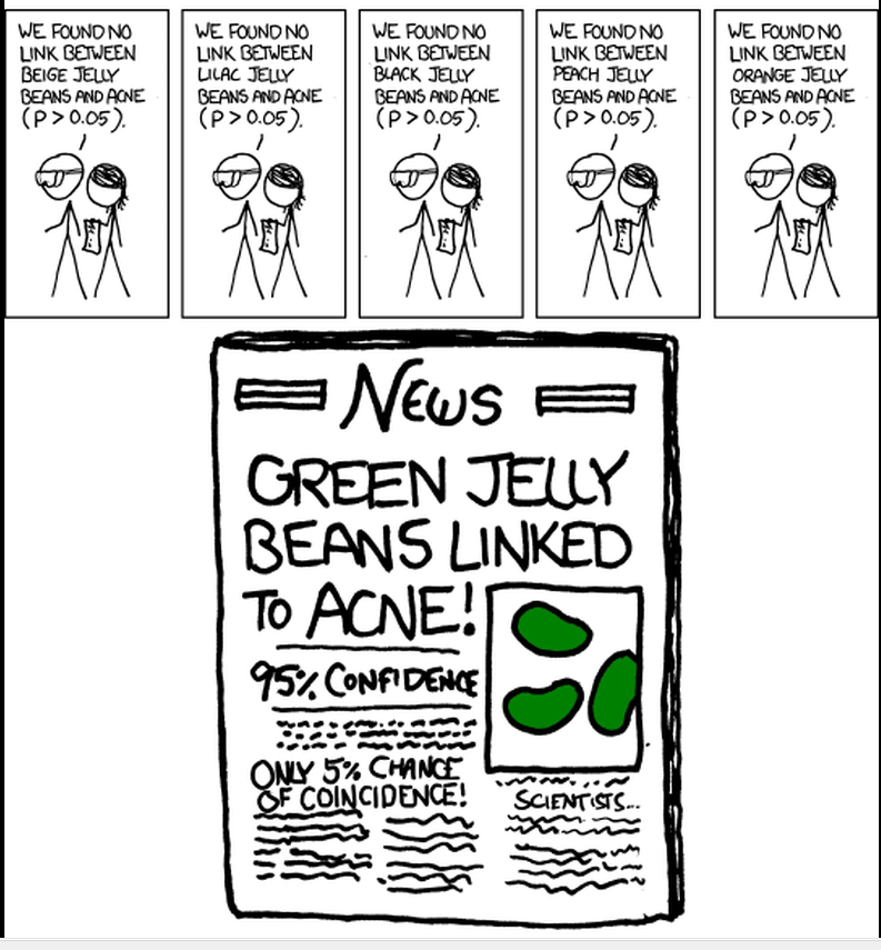
“Why most published research findings are false”

• The multiple testing problem

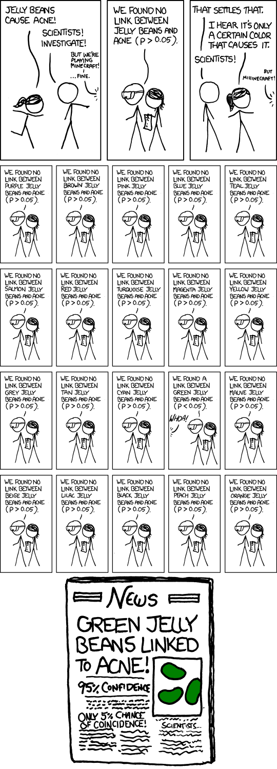
“Why most published research findings are false”

• The multiple testing problem

Unpublished work as Dark Matter

We can only see 5% of the universe.

Analogy with dark matter

Meta-analysis - most of it is trying to estimate the unknown latent variable of what isn’t published

Solutions

Don’t focus on testing a null hypothesis.

Solution is simple

Solutions

Pre-register and publish all results.

but takes time and a shift in culture

But has already happened in medicine

The ASA statement

2016

2019

Stop using p values and “statistical significance”.

Reproducibility Crisis is accepted as mainstream idea

ASA have had had two Special Issues and Statements saying …

But not much has changed

Solutions

• use Bayesian approach (not NH testing)
• change journal policies
• registered reports
  • pre-register experimental design
  • report all results (negative & positive)

Summary

• we confuse measurements with “facts”
• measurements are proxies connected to true process
• usually some form of model involved
• important to recognise uncertainties in the observation process

Summary

Ignoring uncertainties leads to:

• high “false discovery rate”
  • P(claiming to find effect when none present)
• biased results in literature
• the “reproducibility crisis”

Summary

The Bayesian approach:

• avoids null-hypothesis testing
• incorporates prior knowledge \(P(\mathrm{effect})\) or \(P(\theta)\)
• propagates errors explicitly
• use hierarchical models to represent measurement error

Summary

“All models are wrong, but some are useful.”

George Box, 1976.

Summary

“All models are wrong, but some are useful.”

George Box, 1976.

“All data are wrong, but some are useful.”